Welcome to the world of single-cell RNA sequencing (scRNA-seq) analysis! In this Scanpy tutorial, we will walk you through the basics of using Scanpy, a powerful tool for analyzing scRNA-seq data. Whether you are a beginner or just need a refresher, this guide will help you get started with real-world examples and applications.
What is Scanpy?
Scanpy is a Python-based package designed for the analysis and visualization of single-cell RNA sequencing data. It provides efficient algorithms to handle large datasets and is widely used in the research community.
Why Use Scanpy?
- Efficiency: Handles large datasets smoothly, crucial for scRNA-seq analysis.
- Comprehensive: Includes a wide range of tools for preprocessing, visualization, and analysis.
- Community Support: Widely used with extensive documentation, Scanpy tutorials, and an active user community.
Scanpy Tutorial For Beginners
Installing Scanpy
Before we dive into using Scanpy, we need to install it.
Prerequisites
Ensure you have Python installed. We recommend using Python 3.8 or later.
Installation Steps
Using pip: Open your terminal or command prompt and type:
pip install scanpy
Using conda: If you prefer conda, use:
conda install -c conda-forge scanpy
Once installed, you’re ready to start this Scanpy tutorial!
Loading Data
First, we need some data to work with. Scanpy supports various file formats like .h5ad, .loom, and .csv.
Example Dataset
For this Scanpy tutorial, we’ll use a publicly available dataset. Let’s start by importing Scanpy and loading the data.
import scanpy as sc

# Load example dataset
adata = sc.datasets.pbmc3k()
This command loads a dataset of 3,000 Peripheral Blood Mononuclear Cells (PBMCs), a common dataset used in many Scanpy tutorials.
Preprocessing the Data
Preprocessing is crucial for quality analysis. It involves filtering cells and genes, normalizing data, and detecting highly variable genes.
Filtering
We start by filtering out low-quality cells and genes. This ensures that our analysis is not affected by noise.
sc.pp.filter_cells(adata, min_genes=200)
sc.pp.filter_genes(adata, min_cells=3)
Normalization
Next, we normalize the data to make it comparable across cells. This step adjusts for differences in sequencing depth.
sc.pp.normalize_total(adata, target_sum=1e4)
sc.pp.log1p(adata)
Identifying Highly Variable Genes
Identifying highly variable genes is important for downstream analysis as they provide the most information about cell-to-cell differences.
sc.pp.highly_variable_genes(adata, min_mean=0.0125, max_mean=3, min_disp=0.5)
adata = adata[:, adata.var.highly_variable]
Data Visualization
Visualizing data helps in understanding its structure and quality. In this Scanpy tutorial, we will use PCA, t-SNE, and UMAP for visualization.
PCA (Principal Component Analysis)
PCA reduces the data’s dimensionality, making it easier to visualize.
sc.tl.pca(adata)
sc.pl.pca(adata)
t-SNE and UMAP
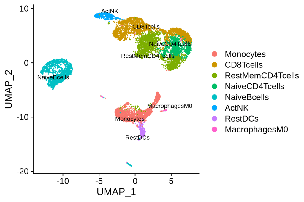
t-SNE and UMAP are popular techniques for visualizing high-dimensional data in 2D. They are particularly useful for identifying clusters of cells.
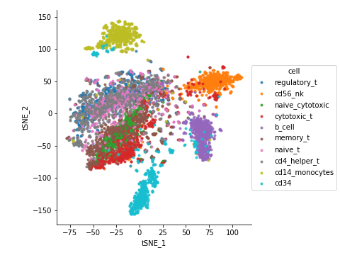
sc.tl.tsne(adata)
sc.pl.tsne(adata)

sc.tl.umap(adata)
sc.pl.umap(adata)
Clustering the Data
Clustering helps in identifying groups of similar cells, which can represent different cell types or states.
Computing the Neighborhood Graph
First, we compute the neighborhood graph. This step prepares the data for clustering.
sc.pp.neighbors(adata)
Clustering
We use the Louvain algorithm for clustering. This algorithm is effective for detecting communities in large networks.
sc.tl.louvain(adata)
sc.pl.umap(adata, color='louvain')
Finding Marker Genes
Marker genes help in identifying the characteristics of each cluster. This is crucial for understanding the biological significance of each cluster.
sc.tl.rank_genes_groups(adata, 'louvain', method='t-test')
sc.pl.rank_genes_groups(adata, n_genes=20, sharey=False)
Congratulations! You’ve completed a basic analysis using Scanpy. This Scanpy tutorial has covered data loading, preprocessing, visualization, clustering, and marker gene identification.
Real-World Applications
In real-world research, Scanpy offers many more advanced functionalities which are used for various applications:
1. Cell Type Identification
Example: Mapping Cell Types in the Human Brain
One of the primary applications of Scanpy is identifying different cell types within a tissue. For instance, in a study mapping the cellular composition of the human brain, researchers used Scanpy to analyze scRNA-seq data from thousands of cells. By clustering the data and identifying marker genes for each cluster, they were able to delineate various neuronal and glial cell types, contributing to a better understanding of brain complexity and function.
Steps in Scanpy:
Data Loading and Preprocessing:
import scanpy as sc
adata = sc.read_h5ad('brain_data.h5ad')
sc.pp.filter_cells(adata, min_genes=200)
sc.pp.filter_genes(adata, min_cells=3)
sc.pp.normalize_total(adata, target_sum=1e4)
sc.pp.log1p(adata)
Clustering and Visualization:
sc.pp.neighbors(adata)
sc.tl.umap(adata)
sc.tl.louvain(adata)
sc.pl.umap(adata, color='louvain')
sc.tl.rank_genes_groups(adata, 'louvain', method='t-test')
sc.pl.rank_genes_groups(adata, n_genes=20, sharey=False)
2. Understanding Cellular Heterogeneity in Cancer
Example: Tumor Microenvironment in Breast Cancer
Scanpy is frequently used to study the tumor microenvironment in cancer research. For example, in breast cancer studies, researchers have used Scanpy to analyze scRNA-seq data from tumor samples. By identifying and characterizing different cell populations within the tumor, such as immune cells, cancer cells, and stromal cells, researchers can understand how these populations interact and contribute to disease progression and treatment resistance.
Steps in Scanpy:
Loading and Preprocessing Tumor Data:
adata = sc.read_h5ad('breast_cancer_data.h5ad')
sc.pp.filter_cells(adata, min_genes=200)
sc.pp.filter_genes(adata, min_cells=3)
sc.pp.normalize_total(adata, target_sum=1e4)
sc.pp.log1p(adata)
Identifying Immune Cell Subtypes:
sc.pp.neighbors(adata)
sc.tl.umap(adata)
sc.tl.louvain(adata, resolution=1.0)
sc.pl.umap(adata, color='louvain')
sc.tl.rank_genes_groups(adata, 'louvain', method='t-test')
sc.pl.rank_genes_groups(adata, n_genes=20, sharey=False)
3. Investigating Immune Responses
Example: Immune Cell Profiling in Viral Infections
In immunology, Scanpy is used to profile immune responses to infections. For instance, during the COVID-19 pandemic, researchers employed Scanpy to analyze scRNA-seq data from patients’ blood samples. This allowed them to identify changes in immune cell populations and gene expression patterns associated with severe disease, providing insights into the immune mechanisms underlying COVID-19.
Steps in Scanpy:
Loading and Preprocessing Immune Data:
adata = sc.read_h5ad('covid19_patient_data.h5ad')
sc.pp.filter_cells(adata, min_genes=200)
sc.pp.filter_genes(adata, min_cells=3)
sc.pp.normalize_total(adata, target_sum=1e4)
sc.pp.log1p(adata)
Comparing Immune Cell States:
sc.pp.neighbors(adata)
sc.tl.umap(adata)
sc.tl.louvain(adata, resolution=0.5)
sc.pl.umap(adata, color='louvain')
sc.tl.rank_genes_groups(adata, 'louvain', method='t-test')
sc.pl.rank_genes_groups(adata, n_genes=20, sharey=False)
4. Studying Developmental Biology
Example: Embryonic Development in Mice
Scanpy is also used to study the differentiation of cells during development. In a study on mouse embryonic development, researchers used Scanpy to analyze scRNA-seq data from embryos at different stages. This helped them trace the lineage of various cell types and understand the molecular mechanisms driving differentiation.
Steps in Scanpy:
Loading and Preprocessing Developmental Data:
adata = sc.read_h5ad('mouse_embryo_data.h5ad')
sc.pp.filter_cells(adata, min_genes=200)
sc.pp.filter_genes(adata, min_cells=3)
sc.pp.normalize_total(adata, target_sum=1e4)
sc.pp.log1p(adata)
Tracing Cell Lineage:
sc.pp.neighbors(adata)
sc.tl.umap(adata)
sc.tl.louvain(adata, resolution=0.8)
sc.pl.umap(adata, color='louvain')
sc.tl.rank_genes_groups(adata, 'louvain', method='t-test')
sc.pl.rank_genes_groups(adata, n_genes=20, sharey=False)
5. Discovering Novel Cell Types
Example: Rare Cell Populations in the Human Lung
In exploratory studies, Scanpy is used to discover novel cell types. For instance, researchers studying the human lung have used Scanpy to analyze scRNA-seq data and identify rare cell populations that were not previously characterized. This can lead to new insights into lung biology and disease mechanisms.
Steps in Scanpy:
Loading and Preprocessing Lung Data:
adata = sc.read_h5ad('lung_data.h5ad')
sc.pp.filter_cells(adata, min_genes=200)
sc.pp.filter_genes(adata, min_cells=3)
sc.pp.normalize_total(adata, target_sum=1e4)
sc.pp.log1p(adata)
Identifying Rare Cell Populations:
sc.pp.neighbors(adata)
sc.tl.umap(adata)
sc.tl.louvain(adata, resolution=1.2)
sc.pl.umap(adata, color='louvain')
sc.tl.rank_genes_groups(adata, 'louvain', method='t-test')
sc.pl.rank_genes_groups(adata, n_genes=20, sharey=False)
Conclusion
Scanpy is a versatile and powerful tool for transcriptomics studies. Its applications range from identifying cell types and understanding cellular heterogeneity in cancer to investigating immune responses and studying developmental biology. The ability to process and visualize complex single-cell data makes Scanpy invaluable for researchers aiming to uncover the intricacies of cellular biology.
By following this Scanpy tutorial and exploring its applications, you can leverage this tool to advance your own transcriptomics research.
Happy Analyzing!!!!

